Zero Shot Forecasting: Chronos vs Toto

Introduction

Good forecasts help with capacity planning and quieter alerts. But one traffic spike or memory leak can make any forecast useless. The goal is simple: prove your forecast beats a naive baseline and stays reliable under uncertainty.

In this post, we compare two forecasting models, Chronos (Chronos‑Bolt) and Toto, on telemetry from Prometheus and OpenSearch. We judge them with two easy metrics: MASE for point accuracy and CRPS for the quality of uncertainty.

Figure: Forecast fan chart for a periodic memory signal (5m aggregation, 256-step horizon). Chronos emits calibrated 0.1–0.9 quantiles.

Long‑horizon forecasts matter for capacity planning. Teams need to anticipate storage growth, provision compute, and schedule scaling windows without constant firefighting. A longer horizon (for example, 256–336 steps) surfaces trend and seasonality far enough ahead to guide procurement, autoscaling policies, and SLO budgets.

Bands, not just point lines, are critical in operations. The quantile envelope translates uncertainty into action: alert thresholds can follow the 0.9 band on spike‑prone services, while budgetary plans anchor around the median or 0.8. When bands widen, you get early warning that risk is rising even if the point forecast looks stable.

A quick note on zero‑shot forecasting

We evaluate both models in a zero‑shot setting used out‑of‑the‑box without fine‑tuning on these specific series. This highlights how well the models generalize to new telemetry without labeled training data. For background, see zero‑shot learning and first part of this blog-post series Zero-Shot Forecasting: Our Search for a Time-Series Foundation Model

What we're forecasting ?

Our dataset comes from the OpenTelemetry Demo (Astronomy Shop), focusing on two common signals:

• Prometheus memory utilization aggregated at 10s, 5m, and 10m
• OpenSearch CPU utilization aggregated at 10s, 5m, and 10m

Forecasting in observability is hard. Real systems are bursty, undergo regime shifts, and only sometimes show seasonality. Some series like Prometheus memory at 5m/10m show clear cycles and relatively stable behavior. Others like OpenSearch CPU are heavy‑tailed and spike‑prone, with outliers that can dwarf the average. Ignore these realities and you get pretty charts with inaccurate results.

A quick exploratory data analysis confirmed it. Memory at 5m/10m looked periodic and well‑behaved, while OpenSearch CPU showed high variability, extreme kurtosis (many tail events), and frequent outliers. Two very different forecasting problems.

Quick EDA (Exploratory Data Analysis) highlights

• Memory (5m/10m): moderate variability (CV ≈ 0.31), clean cycles, near‑zero outliers; stable within operational bounds.
• CPU (5m): highly volatile (CV ≈ 0.48) with frequent extremes and occasional near‑zero segments; heavy‑tailed and spike‑prone.
• 10s windows (both signals): weaker periodicity and more noise; expect broader uncertainty bands.

Dataset quantitative snapshot (selected series)

How to read this:

• CV (coefficient of variation) compares variability across series; higher CV means harder to forecast.
• Kurtosis and outlier percentage signal tail risk; expect CRPS to matter more when these are high.
• Weak trends and low R² suggest regime shifts or noise dominate, so prefer shorter horizons.

The metrics that matter

MASE: Mean Absolute Scaled Error (point accuracy)

MASE compares your model's absolute errors to a naive benchmark. It's scale independent and easy to interpret:

• MASE = 1 → as good as naive
• MASE < 1 → better than naive
• MASE > 1 → worse than naive

In this study, we compute MASE using sktime’s mean_absolute_scaled_error with sp=1 (non‑seasonal). This implicitly benchmarks against a one‑step naive baseline: the forecast at time t equals the observed value at t‑1. Our input is univariate per series, and we provide y_train for each rolling origin. MASE < 1 means the model beats the naive baseline.

Implementation note

mean_absolute_scaled_error(y_true, y_pred, y_train=y_train, sp=1)

CRPS: Continuous Ranked Probability Score (probabilistic accuracy)

CRPS evaluates the entire predictive distribution against the observed value. Lower is better. While MASE gauges the central forecast, CRPS rewards calibrated uncertainty, exactly what SREs need for risk‑aware alert thresholds and error budgets. In production, aim for MASE < 1 and CRPS at or below the naive baseline. Sharp but overconfident distributions are hazardous.

Rule of thumb: Use MASE to prove you've beaten naive; use CRPS to prove your uncertainty is honest.

The models: Chronos vs Toto

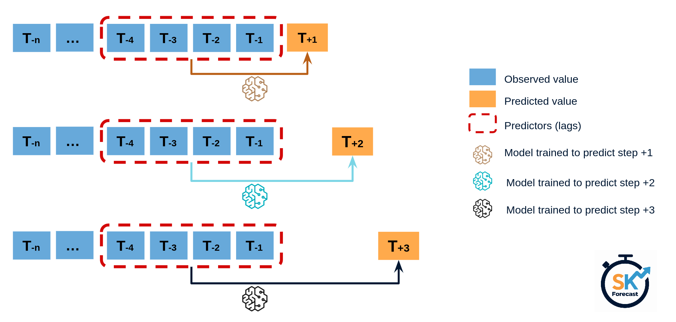
Chronos (Chronos‑Bolt) uses direct multi‑step forecasting: it’s trained to output up to 64 steps in one shot and, in practice, degrades minimally even out to 512 steps. It produces quantiles from 0.1 to 0.9; requesting other quantiles results in errors. The upside: clean fan charts and efficient long‑horizon generation, especially on stable, periodic series.

Toto is autoregressive it generates forecasts step by step, sampling from a parametric distribution at each step. More samples usually mean more stable forecasts and better CRPS—but also higher latency. Toto accepts a parameter called num_samples which dictates the number of samples it should generate to make a forecast. In practice, Toto handled horizons up to 512 steps without issue. Across much of our test data, smaller num_samples (=32) often performed best—reducing inference time (from ~9× slower to ~5× slower as compared to Chronos bolt base) without sacrificing accuracy. Treat this as a solid starting point, then tune as needed.

Experimental setup

• Series & windows: Prometheus memory (10s/5m/10m) and OpenSearch CPU (10s/5m/10m)
• Forecast horizons: 64, 128, 256, and 336 steps
• Baseline for MASE: sktime mean_absolute_scaled_error with sp=1 (non‑seasonal, naive last‑value baseline: forecast at time t equals observed at t‑1); input is univariate; y_train provided per rolling origin
• Hardware: RTX 4060 Notebook GPU (8GB VRAM)
• Metrics: MASE for point accuracy; CRPS for calibrated uncertainty
  • Chronos: default quantiles (0.1–0.9) for fan charts
  • Toto: varied sampling; highlight num_samples=32 as a speed/quality sweet spot (increase num_samples to improve CRPS at the cost of latency)
  • Evaluation: rolling forecast origin with a fixed final test window; record latency per horizon

Data and file structure

• Series naming: <metric>_<window>_<source> — for example, mem_util_5m_prometheus or cpu_util_10s_opensearch.

• CSV files: <prediction_length>_<data_used>.csv — for example, 512_mem_util_5m_prometheus.csv.

• Plot folders: <prediction_length>_<data_used>/ — each folder contains two plots: chronos and toto.

• Root paths in this repo: plots live under Forecast Plots and CSVs under CSV Files.

• CSV header dictionary:

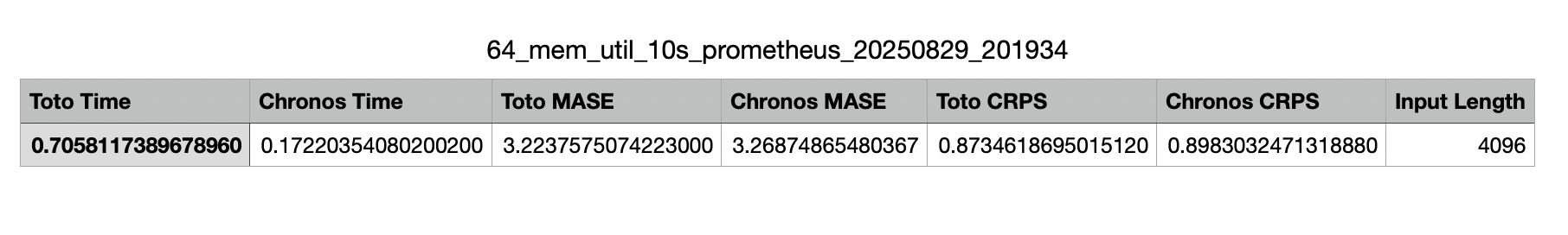
  • Toto Time: Toto inference time for the horizon (ms or s, as exported)
  • Chronos Time: Chronos inference time for the horizon
  • Toto MASE: MASE for Toto’s point forecast vs naïve
  • Chronos MASE: MASE for Chronos’s point forecast vs naïve
  • Toto CRPS: CRPS for Toto’s predictive distribution
  • Chronos CRPS: CRPS for Chronos’s predictive distribution
  • Input Length: Context length used for inference

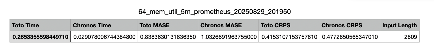
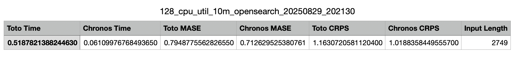
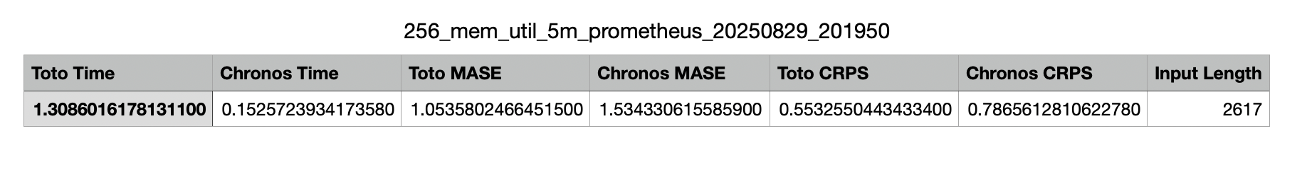
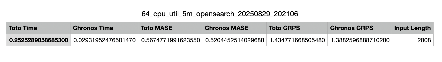
• Example CSVs:

This setup mirrors how you'd actually deploy forecasting in an observability stack: rolling updates, short and long horizons, and guardrails against regression.

All the Forecasting results are available in the GitHub repo.

Results

General observations (zero‑shot): Both models perform well on series with clear cyclic structure (Prometheus memory at 5m/10m) and degrade when periodicity is weak (10s windows, spike‑prone OpenSearch CPU). Use MASE to confirm improvement over naive and CRPS to ensure uncertainty isn’t over‑confident.

Periodic memory (5m/10m)

What you’ll see in the charts: smooth cycles, tight quantile bands, and stable long‑horizon fans.

Term quick guide:

• Smooth cycles: repeating daily/weekly patterns with low random noise; the observed line looks regular and predictable.
• Tight quantile bands: the shaded area around the forecast is narrow, meaning higher confidence and typically lower CRPS. (Chronos uses 0.1–0.9 quantiles.)
• Stable long‑horizon fans: the forecast “fan” stays centered and doesn’t blow up as steps increase (e.g., 256–336). Errors grow slowly and remain bounded.

Metrics: Both Chronos and Toto consistently beat naive (MASE < 1). Chronos often edges ahead at 512‑step horizons thanks to its direct multi‑step design, which keeps error growth in check. CRPS is strong for both, reflecting predictable cycles and well‑calibrated uncertainty.

Figures: Memory utilization, 5m aggregation, 256‑step horizon. Top: Chronos; Bottom: Toto. Bands show 0.1–0.9 quantiles.
CSV:

What this means in ops: Prefer Chronos for long‑range capacity planning on periodic services. Drive alerts from quantile bands (for example, 0.9 for spikes, median/0.8 for budgets) rather than a single point line.

High‑volatility CPU (5m/10m)

What you’ll see in the charts: frequent spikes, asymmetric tails, and wider bands—especially during bursts.

Term quick guide:

• Spikes: sudden, short‑lived jumps in CPU usage, often from traffic bursts or batch jobs.
• Asymmetric tails: the right tail is heavier (big upward moves are more common than equally large drops); CRPS penalizes over‑tight bands here.
• Wider bands: uncertainty grows during bursts; set alert thresholds using upper quantiles (e.g., 0.9) and monitor CRPS.

Metrics: CRPS becomes the deciding factor. Toto can better capture heavy tails with adequate sampling, improving distributional calibration—but with higher latency. Chronos still performs, but if the bands look too narrow on spike‑prone series, be cautious: over‑sharp uncertainty is a red flag.

Figures: CPU utilization (OpenSearch), 5m aggregation, 64‑step horizon. Top: Chronos; Bottom: Toto. Wider bands reflect tail risk.
CSV:

What this means in ops: Increase Toto’s samples when tail risk matters (on‑call noise, error budgets). If latency is a concern, dial back samples or switch horizons. Consider widening alert thresholds to follow the upper quantile band during known burst windows.

High‑frequency 10s windows

What you’ll see in the charts: weaker periodicity, noisier signals, and visibly broader uncertainty.

Term quick guide:

• Noisy signals: high short‑term jitter; individual points carry less meaning, smooth or aggregate when alerting.
• Weak periodicity: little daily/weekly structure; models rely more on short context and degrade faster with horizon.
• Broader uncertainty: wide quantile bands; expect MASE near 1.
• Why short horizons: error compounds across steps; prefer 64‑step horizons for paging and aggregate to 5m/10m for planning.

Metrics: Without strong cyclic structure, both models degrade. Expect MASE ≈ 1 (or marginally better) and wider CRPS. That’s not failure, it’s honest uncertainty.

Figures: Memory utilization, 10s aggregation, 64‑step horizon. Top: Chronos; Bottom: Toto. Bands widen due to weak periodicity.
CSV:

What this means in ops: For near‑term paging, prefer 64‑step horizons and smoothing/aggregation. For capacity planning, use 5m/10m aggregates where structure is clearer.

How to read these figures: the shaded fan shows 0.1–0.9 quantiles; the central line is the median. Tighter shading means lower uncertainty. If the upper band crosses your alert threshold, assume higher risk even if the median stays below it.

How to use the above setup and results?

1. Establish baselines (always do this first)

   • Compute MASE with sktime’s mean_absolute_scaled_error (sp=1, non‑seasonal) using the naive last‑value baseline; provide y_train for each rolling origin; input is univariate per series.
   • No seasonal naive: we do not use seasonal baselines; the metric’s scaling uses last‑value (sp=1).
   • Gate to proceed: target MASE < 1 by a clear margin (≥10–20%) on stable series.

2. Run both models in parallel - Chronos: use 0.1–0.9 quantiles; generate 64, 256, and 336 steps (longer if needed). Save outputs and latencies. - Toto: start with num_samples=32; record inference latency and accuracy. If tails matter and CRPS looks over‑confident, increase num_samples. {{ ... }}

What this means in ops: For near‑term paging, prefer 64‑step horizons and smoothing/aggregation. For capacity planning, use 5m/10m aggregates where structure is clearer.

How to read these figures: the shaded fan shows 0.1–0.9 quantiles; the central line is the median. Tighter shading means lower uncertainty. If the upper band crosses your alert threshold, assume higher risk even if the median stays below it.

How to use the above setup and results?

1. Establish baselines (always do this first) - Compute MASE with sktime’s mean_absolute_scaled_error (sp=1, non‑seasonal) using the naive last‑value baseline; provide y_train for each rolling origin; input is univariate per series. - No seasonal naive: we do not use seasonal baselines; the metric’s scaling uses last‑value (sp=1). - Gate to proceed: target MASE < 1 by a clear margin (≥10–20%) on stable series.

2. Evaluate and calibrate uncertainty - Track both MASE (point) and CRPS (probabilistic). - Acceptance gates:

   • MASE < 1 for your chosen horizon(s).
   • CRPS ≤ naive and stable across windows (no drift).
   • Coverage check: ~80% of actuals inside the 0.1–0.9 band (by design it won’t be 100%; the point is “not too tight”). - If coverage is low or CRPS rises: widen bands (Chronos, Toto) or increase samples (Toto).

3. Match horizons to decisions

   • Paging/on‑call: prefer 64‑step horizons; alert when the 0.9 quantile stays above a threshold for N consecutive points (e.g., N = 3–5 windows).
   • Capacity planning: use 256–336 steps; plan to the median and budget to the 0.8/0.9 quantile.
   • Executive reports: show median plus bands; avoid single‑line forecasts.

4. Wire alerts to uncertainty, not just the mean

   • Use quantile bands for thresholds (e.g., 0.9 for “high‑risk” services).
   • Page only if both conditions hold for N windows: upper quantile > threshold AND observed is trending up.
   • Add dampening: suspend pages if uncertainty (band width) is rapidly expanding after a deploy.

5. Instrument the forecaster (make it observable)

   • Dashboard by service/window (10s/5m/10m):
     • MASE and CRPS as time series; 7‑day moving averages.
     • Quantile coverage (% of points within 0.1–0.9 band).
     • Inference latency by horizon and model; model version and config (samples/context).
   • Alert on trends, not spikes:
     • MASE ≥ 1 for N consecutive windows.
     • CRPS +25% vs baseline for M windows.
     • Coverage < 70–75% for K windows (over‑tight bands).

6. Safety nets and rollback

   • If MASE worsens or CRPS inflates, automatically fall back to the naive (last‑value) baseline.
   • Temporarily widen alert thresholds to quantile bands (e.g., use 0.9 instead of the mean) until retraining.
   • When noise is high (10s windows), aggregate to 5m/10m for capacity decisions.

7. Data hygiene and drift

   • Monitor missing timestamps, step changes, near‑zero plateaus, and value spikes; backfill or mask before scoring.
   • Watch for regime shifts (deploys/traffic changes) that flip winners; keep baselines alive for quick rollbacks.

8. Save artifacts and make results reproducible

   • Store forecast CSVs and plots.
   • Record horizon, input length, and latency in the CSVs (as in your current headers) so teams can compare runs over time.

Limitations

1. Quantile rigidity in Chronos

• What it is: Chronos only emits quantiles at 0.1, 0.2, …, 0.9. Requests for 0.95/0.99 will fail hence we should use Toto for p95/p99 via sampling.
• Why it matters: Many ops teams page on p95/p99. If you can’t natively emit those, aligning with SLOs and dashboards gets tricky.
• How to spot it: Errors when requesting unsupported quantiles, or charts that “jump” because p95 was approximated from sparse quantiles.
• What to do: (a) Standardize on 0.9 for alerts and budgets, (b) if you must show p95, use monotone interpolation between 0.9 and the median and validate coverage weekly, or (c) use Toto for p95/p99 via sampling.
• Example: For mem_util_5m_prometheus capacity planning, anchor to the median for purchase decisions and keep a “risk band” at 0.9. If leadership asks for p95, publish it with a note on interpolation and prove that ~95% of points fell below it in the last 7 days.

2. Autoregressive drift in Toto

• What it is: Toto forecasts step‑by‑step; small errors accumulate across the horizon (drift), especially on long ranges.
• Why it matters: At 256–336 steps, the mean path can wander and bands can get too wide or, worse, too tight and over‑confident.
• How to spot it: MASE is acceptable at 64 but degrades at 256; CRPS rises with horizon; coverage of the 0.1–0.9 band falls < 70–75%.
• What to do: Shorten horizons for paging; increase samples for tail‑heavy series; re‑anchor with rolling origins; cap context length to improve latency.
• Example: On cpu_util_5m_opensearch, 64‑step predictions keep CRPS low and coverage healthy. At 256 steps, CRPS inflates—bump num_samples (e.g., from 32 to 64) or forecast in two 128‑step segments and re‑seed with observations.

3. Regime shifts are real

• What it is: The data‑generating process changes (deploys, feature flags, pricing, marketing, seasonal events). Yesterday’s winner can lose tomorrow.
• Why it matters: Backtests look great until Black Friday or a noisy release day. Then MASE drifts ≥ 1 and CRPS balloons.
• How to spot it: Breaks in seasonality/cycle shape, step changes in level, sharp coverage drops after a dated event.
• What to do: Annotate deploys and campaigns; run rolling backtests; keep the naive (last‑value) baseline alive; trigger model rotation when drift persists for N windows (e.g., 12–24).
• Example: After a canary deploy, mem_util_10m_prometheus loses its daily dip. Chronos still looks fine at the median, but coverage falls to ~60%. Flip alerts to the baseline temporarily and retrain on post‑deploy data.

4. Non‑periodic, high‑frequency data

• What it is: 10‑second series with little cyclic structure and high jitter; signal‑to‑noise ratio is low.
• Why it matters: Models struggle to beat naive; bands widen; alerts on point forecasts become noisy.
• How to spot it: MASE ≈ 1 across models; CRPS wider than at 5m/10m; frequent threshold crossings that don’t persist.
• What to do: Alert on aggregates (5m/10m), smooth inputs, add exogenous signals (release windows, batch schedules), and cap horizons at 64 for on‑call.
• Example: mem_util_10s_prometheus at 64 steps shows honest wide bands and MASE near 1. Aggregate to 5m for planning (where Chronos beats naive) and keep 10s only for exploratory drilling.

Conclusion

If you remember only two things, make them these:

MASE tells you if your point forecast truly beats naive. CRPS tells you if your uncertainty is believable when it matters most.

On periodic series, Chronos often wins, especially at long horizons, thanks to direct multi-step forecasting and clean quantile bands. On spiky, heavy-tailed series, Toto shines when you tune sampling to balance CRPS and latency. Most teams will benefit from using both: Chronos for stable workloads, Toto where tails do the talking.