
One of our customers runs Parseable in production, where their platform handles a large and constantly changing set of resources. Its services emit data volume metrics with labels for the resource, region, node, status and other context from the request path. Over time, a few of those labels reached the low millions of distinct values while read and write traffic continued throughout the day. A label with millions of possible values has high cardinality. Combining those values with the remaining labels and metrics pushed the possible series space beyond 100 million.
Without those labels, the team could see the total data volume across the platform but could not tell which resources were producing it. Keeping those labels lets the team ask for the top X resources during a time window. However, answering that question still requires looking across every active resource in the window, calculating a rate, grouping the values and ranking them. Across the complete metric stream, this deployment operates at around 100 million distinct time series within a minute. Dropping those labels would reduce cardinality, but it would also remove the fields needed to answer the question. The team needs those dimensions, so dropping them is not an answer. That is the production problem behind this blog.
Why this workload creates so many series
A traditional time series database treats the time series as the main storage object. A sample comes in, the database finds the series it belongs to, and the sample is appended to that series. In this widely used data model, the metric name and the complete label set identify a series. This sample belongs to one series:
resource_data_bytes_total{resource_id="resource-a", region="us-east-1", node="node-17"}Changing only the resource creates another series:
resource_data_bytes_total{resource_id="resource-b", region="us-east-1", node="node-17"}Changing the node creates another one again. The same thing happens with region, status, or any other label on the metric. If a single metric has millions of possible resource values, that label can already create millions of series. Add the other dimensions and the count multiplies. The database is not only storing samples. It is also creating, indexing, and managing the series identities produced by those combinations.
The query behind the question looks like this in spirit, using 20 as one example of the requested result size:
topk(
  20,
  sum by (resource_id) (
    rate(resource_data_bytes_total[1h])
  )
)
That query returns 20 results, but topk is the last part of the work rather than the first. A series-first TSDB has to find every matching series for resource_data_bytes_total, read and decode the samples in the requested window, calculate the rate for each series, group those results by resource_id, and rank the grouped values. Region, node, status, and other labels can make many series contribute to the same resource. Changing the requested result from 20 to 10 does not reduce the matching series that must be evaluated before the ranking can happen. The output is small while the input and the intermediate state can still be very large.
For this model, a new label combination means new series state and new index entries. Recent samples need memory or local storage. Older samples move through blocks and compaction. A typical series storage layout keeps an index that maps metric names and labels to series in chunk files. Short lived combinations create churn because each identity still has to be created and indexed even when it appears briefly. Series indexes work well when the label space is bounded and identities repeat often. The cost changes when a label with millions of values keeps expanding the set.
On the query side, the TSDB spends CPU calculating rates and aggregations, memory holding decoded samples and intermediate groups, disk or object storage reads fetching chunks, and network bandwidth when the query fans out across nodes. More matching series generally means more work before the requested values are known. Distributed TSDBs often use sample, chunk, and per-query memory limits to stop one broad query from taking over a query node. At this scale, the same query can take longer or reach those limits even though the response is only a few rows.
Sharding can spread the calculation across more query nodes, caching can help when the same request repeats, and recording rules can precompute a known aggregation. Each option is useful, but none removes the underlying work. Sharding still reads and merges the matching data, caching helps only after a result exists, and a recording rule spends compute and storage ahead of time for a question chosen in advance. High cardinality therefore shows up as more than stored sample volume. It becomes index growth, active series memory, compaction work, query fan out, and longer query execution. If the immediate problem is an existing Prometheus deployment, use the Prometheus cardinality runbook to find the metrics and labels creating the series growth.
What changes when labels are columns
Columnar time-series storage changes the physical layout of the same metric data. You can still think of each sample as a row, but values from the same field are stored together. Timestamps sit with timestamps, metric names with metric names, values with values, and resource identifiers with resource identifiers. The high cardinality field has not disappeared. It is kept as a column that can be read when a query asks for it.
| timestamp | metric_name | value | resource_id | region | node | service | status |
|---|---|---|---|---|---|---|---|
| 10:00:00 | resource_data_bytes_total | 1824 | resource-a | us-east-1 | node-17 | ingest-api | 200 |
| 10:00:01 | resource_data_bytes_total | 948 | resource-b | us-east-1 | node-17 | ingest-api | 200 |
With that layout, another resource identifier is stored as another value in its column. The column can still contain millions of distinct values, and grouping by it still takes work, but the physical layout no longer has to revolve around a long lived object made from the complete metric and label combination. The dimensions stay in the data while the storage model changes where their cost appears. Putting values from the same field together also gives encoders and compression codecs more similar data to work with. Repeated metric names, regions, status values, timestamps, and other fields can be represented more compactly than a row format that repeats the complete record for every sample. Fewer stored bytes reduce the storage footprint, the amount transferred from object storage, and the cost of retaining the data for longer periods.
Look again at the ranking query. The calculation needs the requested time range, metric name, sample value, resource_id, and the labels required to keep the rate calculation correct. It does not need every label column just because those labels exist in the dataset. A columnar reader can project the fields used by the query and leave the rest on storage. When a query does not filter or group by resource_id and the plan does not otherwise require it, the reader can leave that column on storage. Reading and decoding fewer bytes reduces CPU, memory, storage I/O, and network transfer along the query path.
Columnar storage does not make the high cardinality calculation disappear. Ranking resources still means reading matching identifiers, calculating rates, grouping results, and sorting the groups. The difference is that the cost is paid by queries that use the dimension instead of being attached to every possible series during ingestion. Parseable builds on this layout and uses parquet metadata and object storage to narrow the files and byte ranges that reach the aggregation stage.
How Parseable uses Apache Parquet
Parseable keeps durable telemetry in S3-compatible object storage. Incoming metrics are staged locally in an Apache Arrow-based format, then background jobs convert them into compressed Apache Parquet files. The files keep labels as columns and split rows into row groups and pages. What makes Parquet useful here is the file footer. It sits at the end of the file and carries the schema, row group layout, column locations, encodings, and available statistics.
The footer lets a reader answer a few questions before it reads the data itself. It can find the row groups in the file, the columns that are present, available minimum and maximum values for a column chunk, and the byte ranges that contain the required columns. For an hour-long query, this can avoid fetching and decoding parts of an object that cannot contribute to the result.
Parseable adds another layer before the parquet reader opens a file. When a parquet file is produced, Parseable records its time bounds, row count, size, column statistics, and sort order in a manifest. Snapshots point the query path to the manifests that are visible for a stream. A query for the last hour can remove files outside that window before parquet reading begins.
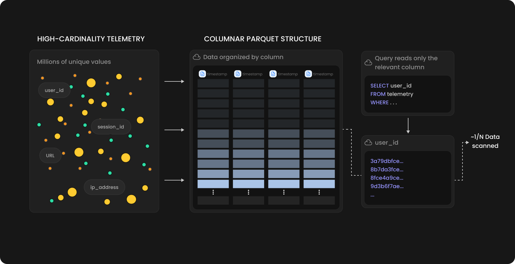
For OpenTelemetry metrics, Parseable writes parquet in a metric-friendly order. Rows are sorted by metric name and timestamp. The sort order is written into parquet metadata, and a bloom filter is enabled on the metric name column. Then a query for one metric gets a narrower path through the data than a scan across every metric in the file.
The query gets several chances to stop early. The time range narrows snapshots and manifests. Manifest statistics narrow files. The parquet footer narrows row groups and columns. The bloom filter can reject row groups that do not contain the requested metric. Page statistics can reduce the read further inside a matching row group. None of this requires Parseable to know every resource identifier in advance. The system first asks whether a file, row group, or page can contain the metric and time range being queried. If the answer is no, that data stays on object storage.
This is where the query cost changes. Less data fetched from object storage means fewer bytes moving over the network. Column projection and data skipping mean fewer values to decode and less memory used before aggregation begins. The exact saving depends on the query and the data distribution. A broad query that matches every row will read more than a selective query, but parquet gives the query engine several places to remove unrelated data before spending CPU on it.
How Parseable handles high-cardinality metrics at scale
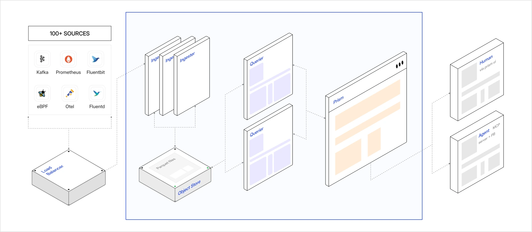
The deployment in this story sends metrics through OpenTelemetry Collectors running across regions. Collector exporters batch telemetry and hold their own queues before the data reaches Parseable, so exporter batch size and queue size live before Parseable receives the request. Once a batch arrives, the ingestor validates it, flattens the OpenTelemetry metric payload into columns, builds Arrow record batches, and writes those batches to local staging. The ingestor then acknowledges the request without waiting for parquet conversion or object storage upload. This keeps CPU-intensive conversion and network-intensive upload out of the collector request path while ingestion continues with incoming batches.
The stream writer stores compressed Arrow IPC files in local staging. Staging gives Parseable enough rows to build useful parquet row groups instead of creating tiny objects for every incoming collector batch. Larger row groups give encodings, statistics, and bloom filters more data to work with. Local sync then takes closed Arrow files from staging, groups compatible data, handles schema changes, and writes parquet through a temporary file. For metric streams, each row group is sorted by metric name and timestamp before the file is made final.
Object-store sync uploads completed parquet files. Uploads can run concurrently and larger files can use multipart upload. Parseable verifies the uploaded object and builds a manifest entry from the file metadata. That entry carries the file location, row count, sizes, column statistics and sort order. The snapshot is updated only after conversion and upload complete. This makes the file visible to query nodes. Init sync handles ordinary failure cleanup around this flow. If an ingestor stops with unfinished staged or temporary files, valid staged data can be made available for processing again and empty invalid files can be removed.
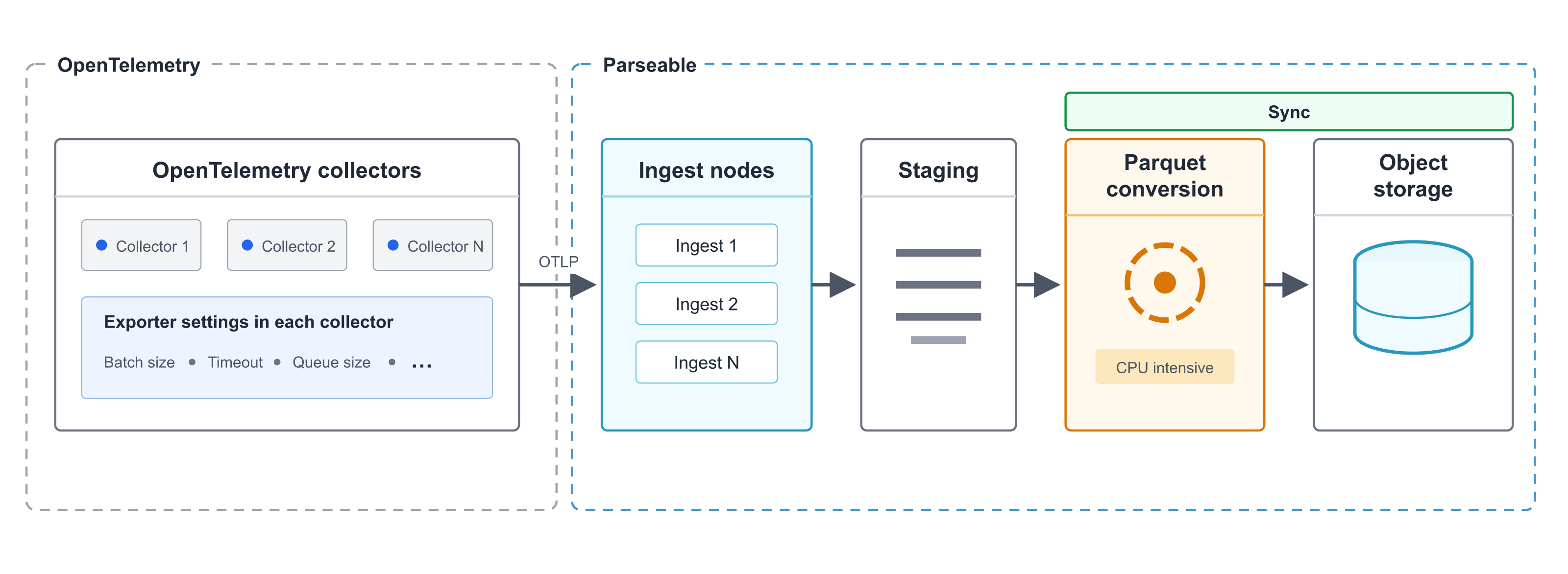
A parquet object becomes part of the queryable set only after the write, upload, verification, manifest update and snapshot update are done. By the time metric data lands in object storage, it has passed through staging, parquet conversion, compression, upload and manifest update. Parseable reduces the metric data size by around 90% and more with parquet, although the exact reduction depends on schema, repeated label values and the distribution of metric values. At this ingest rate, reducing the stored volume directly reduces object storage use and the cost of keeping a longer history.
Now take the ranking query from the beginning. The one hour time filter first selects snapshots and manifests that overlap that window. File-level statistics remove parquet files that cannot satisfy the metric and time predicates. For the remaining files, the parquet reader fetches footer metadata and checks row groups. The bloom filter on metric name can reject a row group that does not contain resource_data_bytes_total. Since rows were sorted by metric name and timestamp during conversion, page statistics can lead the reader to a smaller part of a matching row group.
Column projection controls the next step. For this query, the plan needs metric samples, timestamps, resource identifiers, series identity, and the labels required to preserve the calculation. The query engine calculates the rate for matching series, sums the result by resource_id, and keeps the 20 highest values requested in this example. Parseable still has to aggregate every matching resource value. If all rows in the hour belong to the requested metric, the aggregation still has to process them. The architecture removes unrelated time ranges, files, metrics, row groups, pages, and columns before that work begins.
That reduction lowers operating cost as well as query time. Query nodes decode fewer unrelated columns and retain less rejected data in memory. They also transfer fewer bytes from object storage. Ingestors stage the metric stream without building a historical in memory map of every label combination while background jobs produce ordered and compressed parquet files. Manifests and parquet footers narrow each query to the files, columns and rows that can answer it while keeping high cardinality labels available without making every combination the center of the storage design.
Final thoughts
High cardinality is not bad by nature. It is what systems look like when they scale and when teams start asking better questions from their telemetry. In this workload, a resource identifier was needed to find where activity was concentrated. In another system it may be customer, pod, route, build, device, region, or anything else that explains what changed. Those labels are not noise just because they create more combinations. Removing them may also remove the answer someone needs during an incident next month.
The storage system should not force that choice during ingestion. A series-first TSDB usually pays when it creates, indexes, and manages each series. Parseable keeps those labels in columns, uses manifests and parquet metadata to remove data that cannot match, and spends the remaining work on queries that use those labels. A query that groups by a high cardinality field still pays for that grouping, but a query that does not use the field does not carry the same read cost. The user decides when a dimension is useful instead of the storage model deciding that it should never have been kept. The high-cardinality observability solution covers the product architecture and evaluation path.
Many series-first storage models were designed when telemetry volumes and label spaces were smaller. That does not make those systems wrong, but it does mean their assumptions can become limited and expensive as workloads change. Systems now produce more dimensions, teams keep more history, and AI gives operational data more uses than it had a decade ago. Treating every workload through the same rule and telling every team to drop high cardinality labels ignores why those labels were added in the first place.
Object storage changes the retention and ownership side too. Telemetry can stay in S3-compatible storage inside the team's account and under its access and retention policies. Older data does not have to remain on local disks attached to every query or ingestion node. Keeping five years of telemetry still has a storage cost, but compression and object storage give it a different cost model from keeping five years of hot database state. Compute can scale around ingestion and query demand while object storage remains the durable layer.
The user should decide which labels to keep and when to query them. The tool should carry those dimensions instead of asking people to discard them because its storage model was built for the workloads of the previous decade.